Mining Tweets in Python - the Bieber Fever
During my PhD a fellow postgrad student joked that finite element analysis was really all about the pretty pictures. My last few blog entries were a little code-heavy with no visual relief, so today, we go on the chart-offensive (get it?) and doing a little demo of how to produce a word cloud and bar chart from Twitter using Python. If you haven’t used Python before then this blog post introduces a very useful set of packages to do analysis with. When creating this blog we found the 2nd edition of the book ‘Mining the social web’ an extremely useful resource for tips on accessing and using the Twitter API in Python. The book’s GitHub page is here. I am using the Python Spyder IDE, and running Python on Ubuntu 13.10. Spyder is a nice full featured, cross-platform development environment for Python and we highly recommend it.
Lets define some terms to clear up a potential source of confusion. The Twitter Python package used here is called ‘twitter’. When referring to the package, we will use the lower case ‘twitter’ and the upper case ‘Twitter’ when referring to the service itself. To confuse things further, there is another Python package called ‘python-twitter’ which is loaded in exactly the same way as the ‘twitter’ package but is not the same package. Hopefully pointing out this distinction will prevent any confusion.
In this demonstration, we use both the Twitter search and streaming APIs. The search API is used to collect the first 10,000 tweets of a trending topic in the UK - whatever that happens to be, and the streaming API to aggregate data from Twitter for a period of about 2 hours. Since the public streaming API will only track for specific filtered searches, a high tweet rate filter was required. I am afraid to say that after trying reputable filters such as the financial times, etc. the first high volume filter we found was … wait for it … Justin Bieber. For a long time I only heard about this phenomenon and have successfully avoided having anything to with it, but now I have been forced to contend with it. No matter who you are, the ‘Bieber fever’ gets you in the end some how. Even if you doubt Justin’s contribution to music, I have a strong suspicion that many Twitter app developers test their code on his Twitter stream. While I was preparing the material for this blog entry, I thought that my streaming code was broken till I pointed it at ‘he who must now not be named’ and boom - out gushed all this … stuff, then I realised that other Twitter filters were just taking ages to update.
To be honest till now I haven’t been very excited about Twitter, but there’s something about seeing the information elements of something that piques my interest. When you watch the tweet stream being pulled down, you realise that you are looking at something that approximates to a collective stream of consciousness, and analysing this is interesting.
In this simple demonstration, we create a word count bar chart and a word cloud from the tweets. This is quite basic analysis, but is the first step to analysing this kind of data. We will also investigate the I/O speed of two storage methods, HDF5 and mongoDB using the h5py and pymongo modules. Though HDF5 is a high performance storage method, it is really tuned for numerical data; mongoDB is built on noSQL principles and is used for storing unstructured data. The tweet are stored textually and sequentially from the tweet streams for a period of two hours, we will then see how quickly all the tweets can be retrieved from the respective storage formats.
Analysis
Loading the packages
The packages used this blog are given in the code block below
from pytagcloud import create_tag_image, make_tags
from pymongo import MongoClient
import matplotlib as mp
import pandas as pd
import numpy as np
import twitter
import nltk
import time
import h5py
import re
The pytagcloud package is used to create the word clouds, as described before, pymongo is used for mongoDB I/O, matplotlib is used to create the bar chart of word counts, the pandas package is used to create the frequency table, numpy is there for arrays, the twitter package is used for accessing the Twitter API, the nltk package a Natural Language Tool-Kit that is used here to tag the words to verbs, nouns, etc, the time package is used for timing processes, the h5py package is used for accessing HDF5 I/O functionality and the re package is for regular expressions. What a nice bevy of packages.
Some workhorse functions
In this analysis, there some processes will be used over and over again, so it helps to set these as functions and call them repeatedly later.
This an R-like lapply() function and should go into the littleR theme I created in my previous blog entry. It can be argued that you don’t really need an lapply() function in Python, for me it has been habit forming in R, so I use it here.
def  lapply(_list, fun, **kwargs):
  return [fun(item, **kwargs) for item in _list]
Below are two functions In() and Not(). The In() function is the vectorized in for whether a list of items are in another vector list. The Not() function is a vectorized not for negating a boolean vector.
# Vectorized logic in
def In(vec1, vec2):
  return np.array(lapply(vec1, lambda x: x in vec2))
# Vectorized logic not
def Not(vec):
  return np.array(lapply(vec, lambda x: not x))
The next functions deal with tweet objects from the Twitter API. The purpose of the GetItem() function is to get a specific item from a tweet status object, the GetTrendNames() function obtains the trend names from tweet trend returns and the GetTagWords() functions returns the words from the token pairs obtained from the nltk tagging process. How these work will be clearer later on.
def GetItem(status, item):
  return status[item]
def GetTrendNames(twitterTrends):
  return [index['name'] for index in twitterTrends[0]['trends']]
def GetTagWords(tweetTokenPairs, tagPrefix):
  return [word for (word, tag) in tweetTokenPairs if tag.startswith(tagPrefix)]
The Twitter search API
Before you can start using the Twitter API, you need to register with Twitter (i.e. have a Twitter account) and then go to the developer section and login here to create your Twitter app where you get your API tokens.
Here I create the Twitter instance
# Here you enter your own API keys and tokens
consumerKey = ''
consumerSecret = ''
oauthToken = ''
oauthTokenSecret = ''
auth = twitter.oauth.OAuth(oauthToken, oauthTokenSecret, consumerKey, consumerSecret)
# This creates the Twitter API instance
twitterApi = twitter.Twitter(auth = auth)
The function below downloads tweets from the Twitter search API, it is a modified version of that given the the book Mining the social web 2nd Edition.
# Twitter search function to get a number of tweets using a search query
def TwitterSearch(twitterApi, query, approxCount = 500, **kw):
  searchResults = twitterApi.search.tweets(q= query, count=100, **kw)
  statuses = searchResults['statuses']
  while len(statuses) < approxCount:
    try:
        nextResults = searchResults['search_metadata']['next_results']
    except KeyError, e:
        break
    print str(len(statuses)) + ' results have been downloaded from approximately ' \
        + str(approxCount)
    kwargs = dict([ kv.split('=') for kv in nextResults[1:].split("&") ])
    nextResults = twitterApi.search.tweets(**kwargs)
    statuses += nextResults['statuses'] # cool append notation
    print 'A total of ' + str(len(statuses)) + ' have been downloaded'
  return statuses
This function gets at lease the number of tweets specified by approxCount, the way the search API works, you will always retrieve more tweets than you specify since tweets are loaded in batches. The number of tweets can be limited at the end of the function to the exact required number by setting the length of statuses, but I leave it to the user to do this (I regard it as wasteful if the tweets have already been retrieved).
Next we use the where on earth ID to search for tweets in a particular region, in this case the UK. The Where on earth ID comes from the Yahoo Geoplanet API.
# Where on earth ID
ukID = 23424975
We get the trending topics …
# Get the UK trend
ukTrends = twitterApi.trends.place(_id = ukID)
Then we use our TwitterSearch() function to load tweets from the search API. The trending topic was #FM14xmas.
# The trending topic was #FM14xmas
# Grabbing the statuses from twitter for this trending topic, one at a time
statusOutput = TwitterSearch(twitterApi, query = GetTrendNames(ukTrends)[0], \
        approxCount = 10000)
A little regexp
If you are new to Python programming, the Python HowTos page provides a good introduction to various useful general programming tasks in Python (http://docs.python.org/2/howto/index.html). It is hard to overstate how good python documentation is. When you look at the String Services documentation in Python, it is truly a sight to behold. Clearly a lot of care has been taken to prepare this material, its nice to have decent documentation.
We strip the text and format the tweets
# Getting the tweet text
rawTweets = lapply(statusOutput, GetItem, item = 'text')
rawTweets = lapply(rawTweets, str)
We can then split the tweets using spaces
# Splits the tweets into words
tweetShreds = []
for index in rawTweets:
    tweetShreds += re.split('\s', index)
Then we do some clean-up, throw away hash tags, users, non alphabetical characters, web links, empty items and then convert everything to lower case.
# Throw away the hash tags
tweetShreds = lapply(tweetShreds, lambda x: re.sub('\#.*', '', x))
# Throws away the users
tweetShreds = lapply(tweetShreds, lambda x: re.sub('\@.*', '', x))
# Throw away anything that is not alpha upper or lower case
tweetShreds = lapply(tweetShreds, lambda x: re.sub('[^A-z]', '', x))
# Throw away anything that is a link
tweetShreds = lapply(tweetShreds, lambda x: re.sub('^.*http.*', '', x))
# Removes the empty items
tweetShreds = [index for index in tweetShreds if index != '']
# Convert all to lower case
tweetShreds = lapply(tweetShreds, lambda x: x.lower())
A little natural language processing
I think that it is amazing that there are tools that can give us a hint about the nature of the words and structure of the language that we use.
Next we tokenize our tweet shreds assigning grammar label codes, verbs, nouns etc. to each word. Use the nltk.help.upenn_tagset() function to see all the available tokens and
their descriptions.
# The verbs
verbs = GetTagWords(tweetTokens, 'V')
# Nouns
nouns = GetTagWords(tweetTokens, 'N')
# Adjectives
adjs = GetTagWords(tweetTokens, 'JJ')
Here I show the bar chart for the verbs, the same procedure can be used for the other word types. It is worth drawing your attention to the pd.Categorical() function, this is equivalent to the factor() function in R, and you can set levels just like you can in R.
# First we convert verbs to categorical variables
verbs = pd.Categorical(verbs)
# Then we use the describe function to create a frequency table
freqTable = verbs.describe()
# We don't want low counts coming through
freqTable = freqTable[freqTable['counts'] > 100]
# Filter some unwanted words
freqTable = freqTable[Not(In(freqTable.index, ['sas', 'rudolph', 'ben', 'alan',
                    'be', 'is', 'has', 'dont', 'rt', 'david', 'dwight']))]
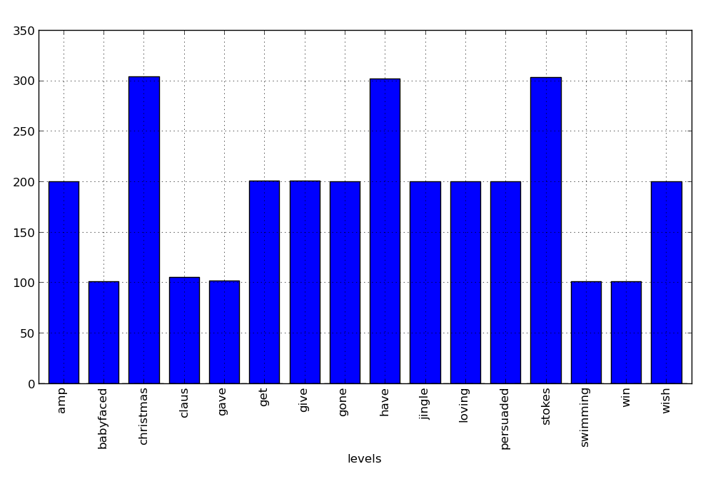
The trendThe trending topic was #FM14xmas - obviously something to do with Christmas, so we expect some related words. Here I create a bar plot of the counts for words with frequency > 100.
# A bar plot of counts
mp.pyplot.figure()
freqTable['counts'].plot(kind = 'bar')
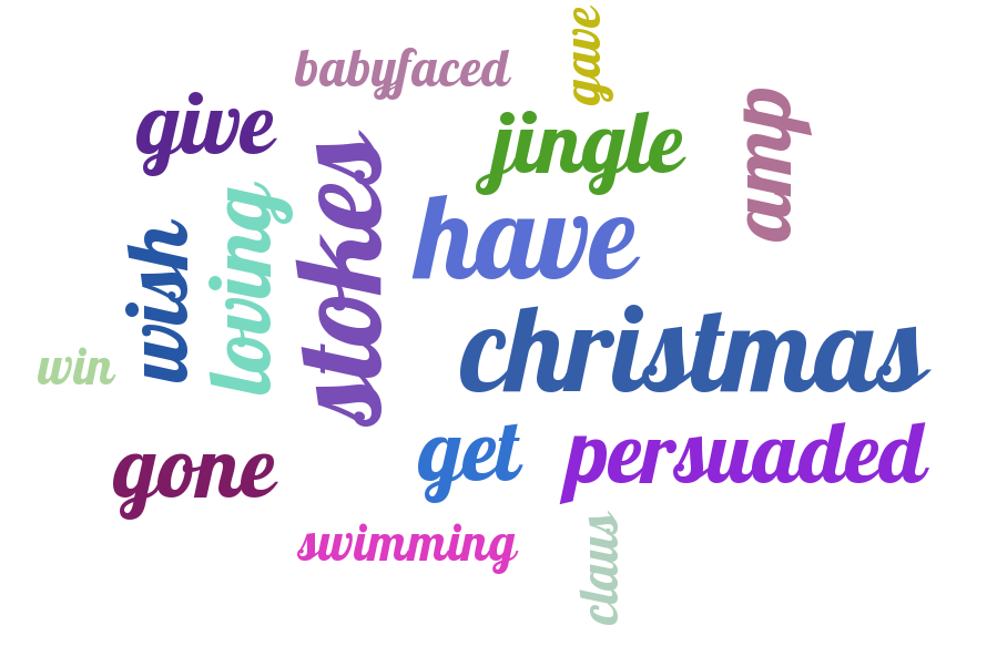
Next I include a word cloud for the verbs
# verbs
verbtags = make_tags(dict(freqTable['counts']).items(), maxsize = 140)
create_tag_image(verbtags, 'wordCloud1.png', size=(900, 600), fontname='Lobster')
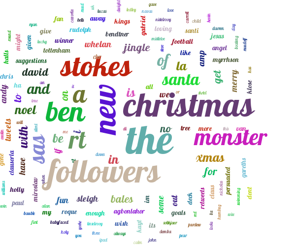
Then the word cloud using all the words
tweetTable = pd.Categorical(tweetShreds).describe()
tweetTable = tweetTable[tweetTable['counts'] > 100]
tweetTags = make_tags(dict(tweetTable['counts']).items(), maxsize = 200)
create_tag_image(tweetTags, 'images/wordCloud3.png', size=(600, 600), fontname='Lobster')
Working with the Twitter stream API
We start by setting up the HDF5 file and mongoDB.
# H5
sTweetH5 = "data/TweetStreams.h5"
tweetH5File = h5py.File(sTweetH5)
h5StreamTweets = tweetH5File.create_group('streamTweets')
# MongoDB
client = MongoClient('localhost', 27017)
# create the database
db = client['tweets']
# Create a collection to write to, this is when the database actually gets created
tweetCollection = db['streaming-tweets']
Notice that there are two separate strategies here, in the HDF5 file, we are saving the tweets to a group called streamTweets and in the mongoDB we are saving the tweets to a collection called ‘streaming-tweets’. There are lots of ways that you can write to HDF5 files. I tried two techniques, the first is simply to write each tweet to its own item in the a group h5StreamTweets but when you try to ready all the tweets back, it is very slow. The second is to treat the tweets as a dataset in the HDF5 file. If you do this you will have to guess the size of the array you need, if you do not guess you have to increase the size of the array dimension periodically this is very very slow. We will present the read-back time associated with reading all the objects from the group and then the read time associated with reading as a dataset.
We first create the twitter stream object:
twitterStream = twitter.TwitterStream(auth=twitterApi.auth)
# See https://dev.twitter.com/docs/streaming-apis
stream = twitterStream.statuses.filter(track = "JustinBieber")
Then we loop through and collect tweets, I did this for about 2 hours
index = 0
ids = []
for tweet in stream:
    tweet = tweet['text'].__str__()
    print tweet
    h5StreamTweets[str(index)] = tweet
    ids.append(tweetCollection.insert({str(index): tweet}))
    print 'Tweet collected @ time: ' + time.ctime()
    index += 1
Now the timings for the reads from mongoDB and HDF5 using groups
# Load the tweets from mongoDB
tA = time.time()
mongoTweets = list(tweetCollection.find())
tB = time.time()
tC = tB - tA
print tC
# 0.207785129547 s
# From HDF5
def GetH5Tweets(x):
    return str(h5StreamTweets[x][...])
tweetNames = lapply(range(0, index), str)
xA = time.time()
h5Tweets = lapply(tweetNames, GetH5Tweets)
xB = time.time()
xC = xB - xA
print xC
# 4.938144207 s
As I said previously, the HDF5 from separate entities in group load is slow, the main difference is that on mongoDB, we can read the whole collection at once, in the HDF5 method we visit each of 38,152 tweets. We can save the tweets as a dataset instead. Lets say that we guess that 40,000 tweets will come down. We create a HDF5 dataset (in a HDF5 file called testH5File) specifying the size and type of the array to be stored. Note that variable string types a tricky in numpy, in fact there isn’t an official variable string type in numpy, these are stored as ‘objects’ so we need to tell HDF5 they variable string type using the notation below
# The variable length data type
dt = h5py.special_dtype(vlen=str)
Then we create the tweet HDF5 dataset.
h5StreamTweets = testH5File.create_dataset('tweets', shape = (40000,), dtype = dt)
My tweets are stored in a list called tweets, I save them to the HDF5 file sequentially (simulating the previous sequential storage in the live tweet stream)
# Now simply turn through the tweets
for ind in range(len(tweets)):
    h5StreamTweets[ind] = str(tweets[ind])
    print 'This is tweet number ' + ind.__str__()
    print tweets[ind]
We get back the lightning fast HDF5 performance we know and love …
xA = time.time()
readTweets = h5StreamTweets[...]
xB = time.time()
# 0.053994178771972656 s
If your data is simple like this, HDF5 should not be ruled out, it is very fast - but you do need to know how much data you want to store. If your data has a complicated document structure, you may be better off with mongoDB or something similar.
Next we create the word cloud as before
# The verbs
verbs = GetTagWords(tweetTokens, 'V')
# Nouns
nouns = GetTagWords(tweetTokens, 'N')
# Adjectives
adjs = GetTagWords(tweetTokens, 'JJ')
#---
# First we convert verbs to categorical variables
verbs = pd.Categorical(verbs)
# Then we use the describe function to create a frequency table
freqTable = verbs.describe()
# Create verb cloud
freqTable = freqTable[freqTable['counts'] > 100]
# Filter some unwanted words
freqTable = freqTable[Not(In(freqTable.index, ['am', 'are', 'be', 'been',
'cant', 'd', 'dgr', 'dont', 'did', 'do', 'dont', 'hi',
'i', 'ilysm', 'im', 'is', 'je', 'justin', 'lt', 'rt',
'yg', 'youre', 'x', 'was', 'were', 'u', 'vo', 'te',
'sla', 'sid', 'featuring']))]
verbtags = make_tags(dict(freqTable['counts']).items(), maxsize = 300)
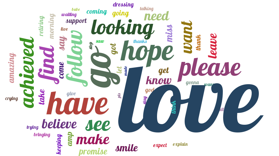
create_tag_image(verbtags, 'images/wordCloudBieber.png', size=(900, 600), fontname='Lobster')
tweetTable = pd.Categorical(tweetShreds).describe()
tweetTable = tweetTable[tweetTable['counts'] > 100]
#tweetTable = tweetTable[Not(In(tweetTable.index, ['rt']))]
tweetTags = make_tags(dict(tweetTable['counts']).items(), maxsize = 200)
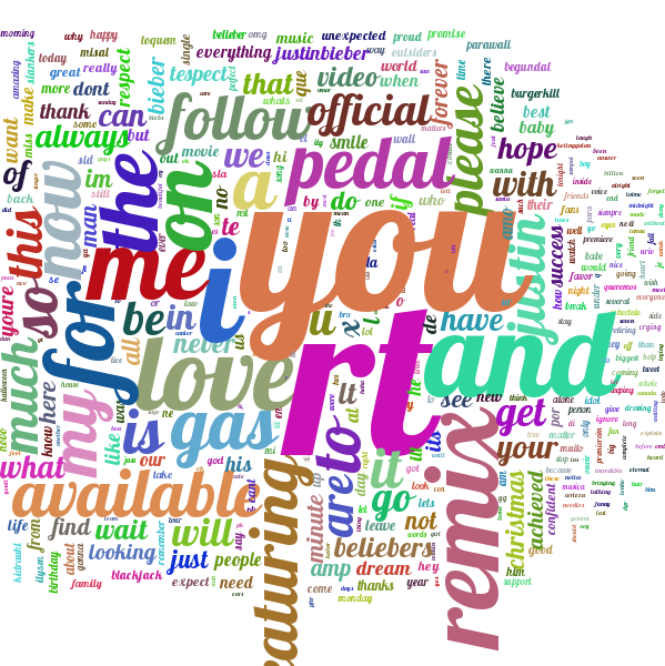
create_tag_image(tweetTags, 'images/bieberCloud.png', size=(600, 600), fontname='Lobster')
The verb word cloud …
and the total word cloud
Summary
Lots of Python packages were used in this blog entry and we only touched on the functionality of each one. These are very powerful packages and they offer lots of functionality for carrying out various processing tasks in Python. The performance and ease of use of mongoDB through pymongo was a pleasant surprise. If HDF5 is used to store noSQL data, much thought needs to be put into exactly how data will be stored to obtain good performance - generally the simpler the data type, the more justified HDF5 format. The twitter Python package is enjoyable to use, it makes pulling tweets from Twitter a straightforward exercise. We made minimal use of pandas package but there is may be more to come in this blog from that package - it has a lot to offer. Regular expressions in Python is straightforward because the documentation is great, even if I don’t use this module in later blogs I will certainly make plenty of use of the module in my work.