R in Engineering Applications: laser profiling example

In this week’s blog, I will look at using R in engineering applications using laser profiling as an example. Some of the material in this article is taken from some work I did back in 2008 part of which involved profiling using lasers at the University of Aberdeen, School of Engineering.

Sometimes there nothing funnier than looking back at code you wrote many years previously, occasionally you surprise yourself at the stuff you were able to do but at other times, your attempts look “cute”, and you realize how much faster/better you could make the code/process. That’s how I felt looking back at my old laser profiling code, but it did the job, and speed was not really a priority in the project.

Below is a picture of the laser profile of the profile of disturbed sand in a flume tank, created using the 3D R plotting package rgl.

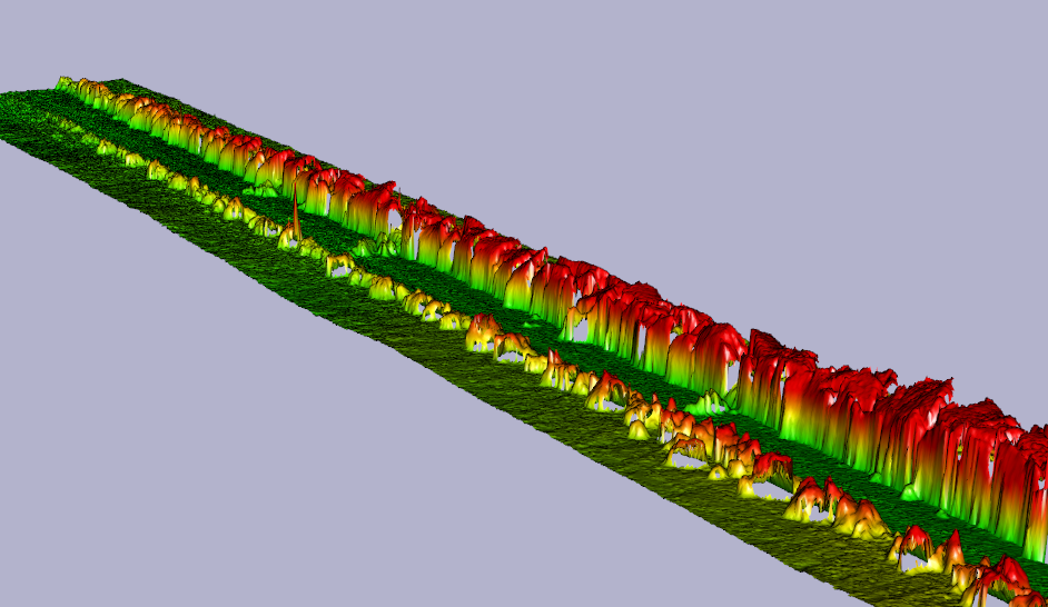
3D Image of laser profile of disturbed sand.

If you are reading this and you are an engineer, it is quite likely that you haven’t heard of R. There are lots of places that you can learn about the history of the language so I will only mention it briefly here. Think of R as being very similar to Matlab, but open source. It comes from the statistics field so the emphasis is a little different but all the important tools are there, in fact most things we need to do in numerical computation are pretty common; whether you are in engineering, genomics, or finance you all still want to invert a matrix, solve differential equations, find Eigen values/vectors of something, and carry out plots. The official website for R is located here.

The experiment

The central idea is quite simple. We have a long flume tank with sand at the bottom; the tank has rails along the sides on the top, and a trolley rides on the rails. Instruments and specimens can be mounted on this trolley. The specimen can be dragged through the sand which disturbs or displaces the sand, after this the specimen is lifted/removed and the laser and camera are mounted on the trolley which then rides over the sand taking the reading of the depth profile. This second process is where the video that will be analysed is recorded.

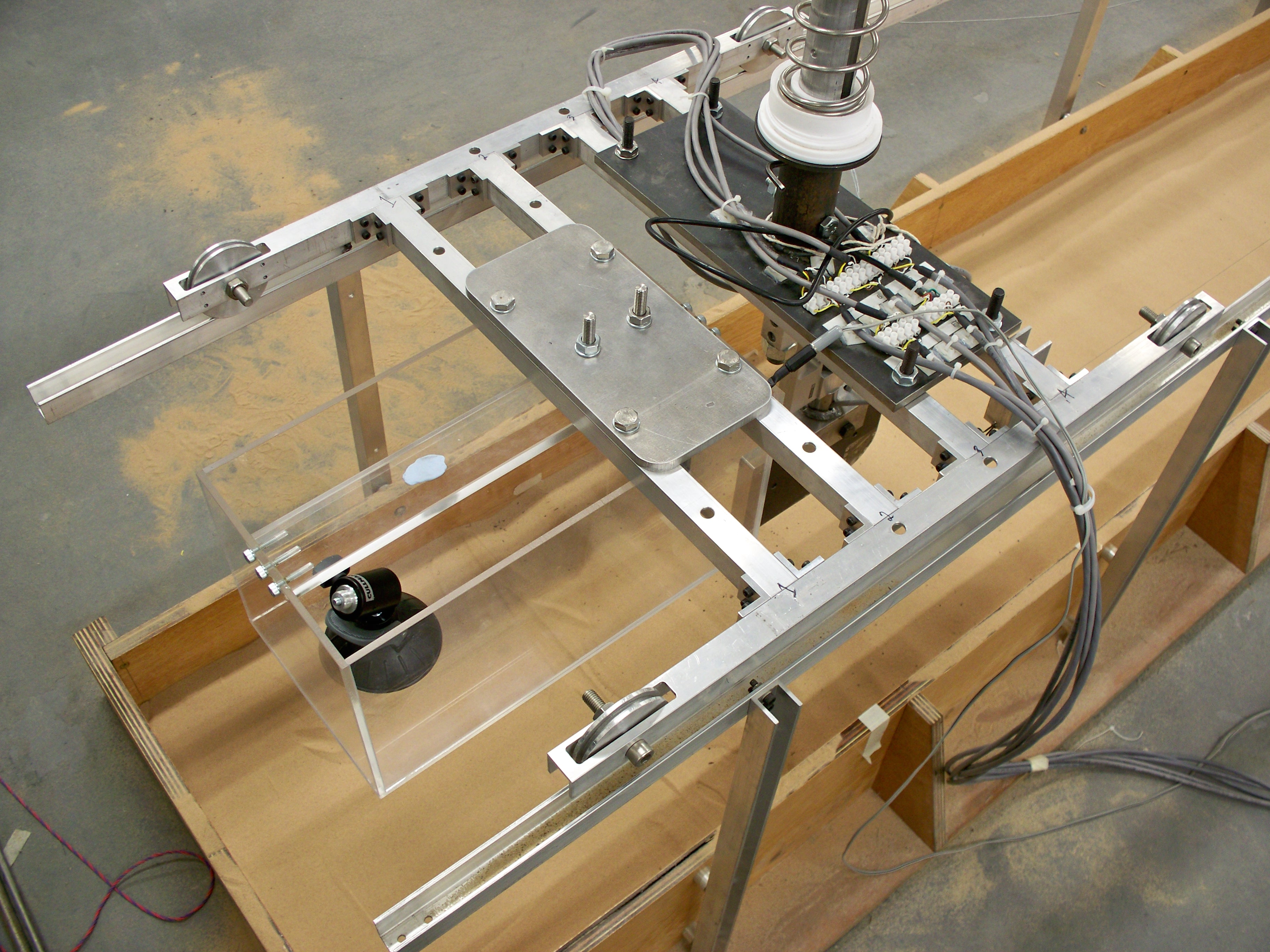
Picture of trolley on tank

Data acquisition

The laser is pretty cheap, you can buy them for about 30 GBP and they produce a line, this line changes shape with the profile of the sand. The digital camera which is also cheap records this image in a video (there’s nothing special about this camera, nowadays, you could probably use your mobile phone to capture a higher pixel density and frame rate than the dedicated camera I used back then, how times have changed – though the lens in a dedicated camera will be better). I actually think that the mounting was the most expensive part of the whole thing because it had to be designed and built. Hey, guess who designed it? I was a dab-hand at Solidworks, those where the days.

Once we record the video, we decompose it to individual picture frames; I used the free software Avidemux to create .jpg stills. The rate of travel of the trolley is constant, we know the frame rate of the camera and the total distance travelled, therefore we know the distance between the frames. The other nice thing about this is that you can pull the trolley as slowly as you want if you want higher resolution along the length of the tank.

The shape of camera lenses means that straight lines are curved in a picture, without going into details, the picture you see from a camera is a distortion of reality, in addition the spatial configuration of the camera with respect to any subjects in the image matters, so to get the true line from the picture of the laser, we need adjust for this by a calibration process.

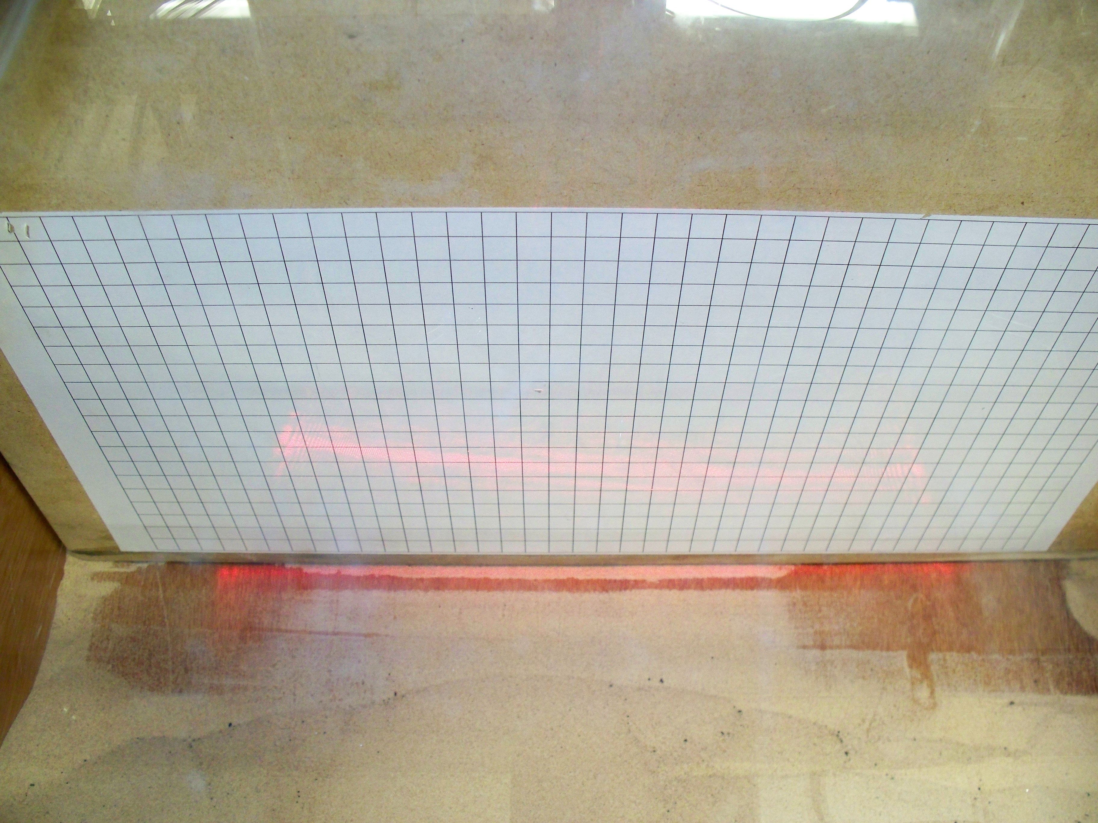
Picture of calibration grid

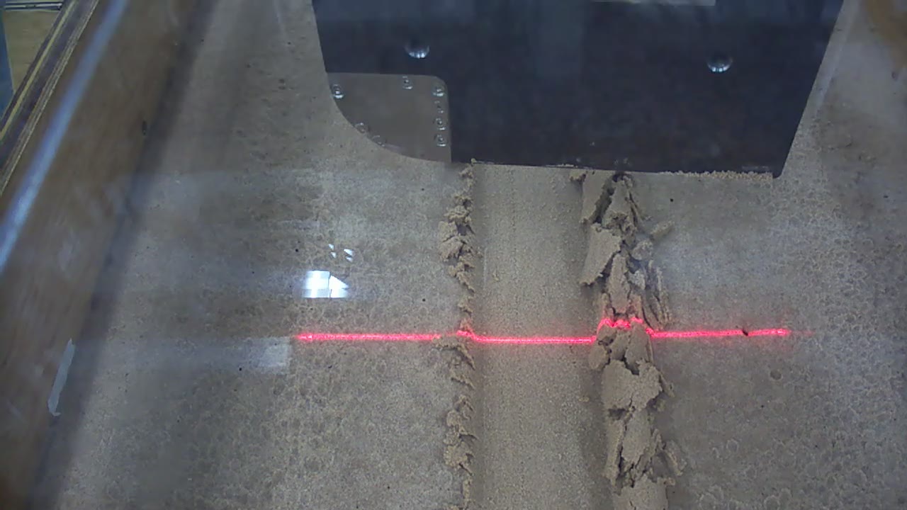
Picture of the laser scanning procedure

Calibration

There are many ways to get the points of intersection of the horizontal and vertical lines from the calibration grid; if interactive graphics are not available you could create a picture of points from an overlay in a graphics package e.g. gimp, and read these points (via the picture) into R. Alternatively in R you could use the interactive locator() function to select and return the points in the picture as x/y numeric values and adjust the coordinates by also selecting the four corners of the picture.

When I was developing the technique however, I chose quite a long winded and tedious way of calibration; I isolated each line in the calibration grid, using a graphics package like gimp drawing splines over the lines into separate picture files. I then found all the points of intersection between the horizontal and vertical lines on the calibration grid as described below.

The separate files each with a single spline picture is loaded into R and then converted into matrices using black/white (0, 255) with the biOps R package. We can then take each horizontal and vertical line combination from the grid, fit curves to them, and find their intersection points in image space. Once we have these points and their analogues in real space, we can obtain coefficients of the equations given by Darboux and Huang and use these to map any future points from image space to real space.

The video with the laser line is done in while the lab is in semi darkness – dark enough to allow us to easily isolate the laser line but light enough so we don’t trip over anything! We use the biOps package again to isolate the red (in this case) laser line and convert all the isolated pixels to points in real 2D space. When we do this for all the pictures, we soon end up with a 3D cloud of points isolated from each of our 2D slices. We also use a smooth to obtain a single line from all the points in the 2D shot.

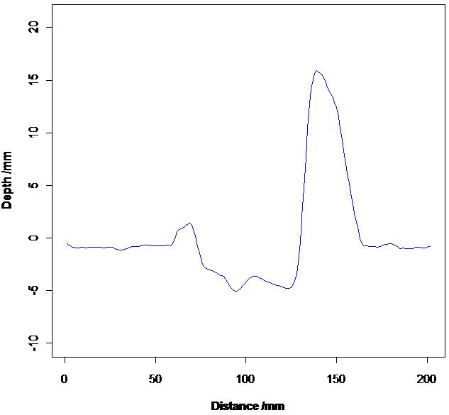
There are lots of options for 3D plotting in R, we can use the rgl package, which allows dynamic interaction with the graphic object, we can also use surface and contour plots, as well as 3D point clouds.

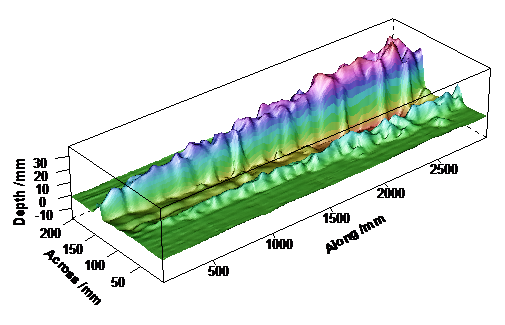
Smoothed 3D plot of profile

Conclusion

Matlab is a fine tool for engineering applications, especially if you are using tool boxes such as Simulink and some very specialist items that may not be readily available elsewhere. However I think that engineers who use Matlab should take R seriously especially if you have to write a lot of code. When it comes down to it R and Matlab are very similar tools but R is open and has a large contributor base, for instance CRAN has well over 4000 packages. Over the last few years it has taken huge strides with respect to speed, parallel processing, big data handling and the ability to be integrated with many other programming languages (C/C++, FORTRAN, Python, Java etc) and platforms (Windows, Mac, Linux, Unix). I think that engineers have a lot to gain from using R as an analysis engine. If you are worried about specialized file formats, there are many R packages that are likely to cater for your needs either on CRAN, or Bioconductor. Don’t let the fact that Bioconductor is aimed at genomic research prevent you from using any of the packages there for your own projects. For instance, the rhdf5 package on Bioconductor will still interface with hdf5 files regardless of the application.

References

1. Darboux F. and Huang C., An Instantaneous-Profile Laser Scanner to Measure Soil Surface Microtopography, Soil Sci. Soc. Am. J. 67:92–99 (2003).